Why Haskell Matters
Abstract
With Haskell, you don’t solve different problems. But you solve them differently.
In this article I try to explain why Haskell keeps being such an important language by presenting some of its most important and distinguishing features and detailing them with working code examples.
The presentation aims to be self-contained and does not require any previous knowledge of the language.
The target audience are Haskell freshmen and developers with a background in non-functional languages who are eager to learn about concepts of functional programming and Haskell in particular.
Table of contents
- Introduction
- Functions are first class
- Pattern matching
- Algebraic Data Types
- Polymorphic Data Types
- Immutability
- Declarative programming
- Non-strict Evaluation
- Type Classes
- Conclusion
Introduction
Exactly thirty years ago, on April 1st 1990, a small group of researchers in the field of non-strict functional programming published the original Haskell language report.
Haskell never became one of the most popular languages in the software industry or part of the mainstream, but it has been and still is quite influential in the software development community.
In this article I try to explain why Haskell keeps being such an important language by presenting some of its most distinguishing features and detailing them with working code examples.
The presentation aims to be self-contained and does not require any previous knowledge of the language. I will also try to keep the learning curve moderate and to limit the scope of the presentation; nevertheless this article is by no means a complete introduction to the language.
(If you are looking for thorough tutorials have a look at Haskell Wikibook or Learn You a Haskell
Before diving directly into the technical details I’d like to first have a closer look on the reception of Haskell in the software developers community:
A strange development over time
In a talk in 2017 on the Haskell journey since its beginnings in the 1980ies Simon Peyton Jones speaks about the rather unusual life story of Haskell.
First he talks about the typical life cycle of research languages. They are often created by a single researcher (who is also the single user), and most of them will be abandoned after just a few years.
A more successful research language might gain some interest in a larger community but will still not escape the ivory tower and typically will be given up within ten years.
On the other hand we have all those popular programming languages that are quickly adopted by large numbers of developers and thus reach “the threshold of immortality”. That is the base of existing code will grow so large that the language will be in use for decades.
A little jokingly he then depicts the sad fate of languages designed by committees by flat line through zero: They simply never take off.
Finally, he presents a chart showing the Haskell timeline:
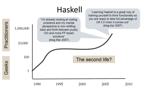
The development shown in this chart seems rather unexpected: Haskell started as a research language and was even designed by a committee; so in all probability it should have been abandoned long before the millennium!
Instead, it gained some momentum in its early years followed by a rather quiet phase during the decade of OO hype (Java being released in 1995). And then again we see a continuous growth of interest since about 2005. I’m writing this in early 2020, and we still see this trend!
Being used versus being discussed
Then Simon Peyton Jones points out another interesting characteristic of the reception of Haskell in recent years: In statistics that rank programming languages by actual usage Haskell is typically not under the 30 most active languages. But in statistics that instead rank languages by the volume of discussions on the internet Haskell typically scores much better (often in the top ten).
So why does Haskell keep being a hot topic in the software development community?
A very short answer might be: Haskell has a number of features that are clearly different from those of most other programming languages. Many of these features have proven to be powerful tools to solve basic problems of software development elegantly.
Therefore, over time other programming languages have adopted parts of these concepts (e.g. pattern matching or type classes). In discussions about such concepts the Haskell heritage is mentioned and differences between the original Haskell concepts and those of other languages are discussed. Sometimes people feel encouraged to have a closer look at the source of these concepts to get a deeper understanding of their original intentions. That’s why we see a growing number of developers working in Python, Typescript, Scala, Rust, C++, C# or Java starting to dive into Haskell.
A further essential point is that Haskell is still an experimental laboratory for research in areas such as compiler construction, programming language design, theorem-provers, type systems etc. So inevitably Haskell will be a topic in the discussion about these approaches.
In the following sections we will try to find the longer answer by studying some of the most distinguishing features of Haskell.
Functions are First-class
In computer science, a programming language is said to have first-class functions if it treats functions as first-class citizens. This means the language supports passing functions as arguments to other functions, returning them as the values from other functions, and assigning them to variables or storing them in data structures.[1] Some programming language theorists require support for anonymous functions (function literals) as well.[2] In languages with first-class functions, the names of functions do not have any special status; they are treated like ordinary variables with a function type.
quoted from Wikipedia
We’ll go through this one by one:
Functions can be assigned to variables exactly as any other values
Let’s have a look how this looks like in Haskell. First we define some simple values:
-- define constant `aNumber` with a value of 42.
aNumber :: Integer
aNumber = 42

-- define constant `aString` with a value of "hello world"
aString :: String
aString = "Hello World"
In the first line we see a type signature that defines the constant aNumber to be of type Integer.
In the second line we define the value of aNumber to be 42.
In the same way we define the constant aString to be of type String.
Haskell is a statically typed language: all type checks happen at compile time. Static typing has the advantage that type errors don’t happen at runtime. This is especially useful if a function signature is changed and this change affects many dependent parts of a project: the compiler will detect the breaking changes at all affected places.
The Haskell Compiler also provides type inference, which allows the compiler to deduce the concrete data type of an expression from the context. Thus, it is usually not required to provide type declarations. Nevertheless, using explicit type signatures is considered good style as they are an important element of a comprehensive documentation.
Next we define a function square that takes an integer argument and returns the square value of the argument:
square :: Integer -> Integer
square x = x * x
Definition of a function works exactly in the same way as the definition of any other value.
The only thing special is that we declare the type to be a function type by using the -> notation.
So :: Integer -> Integer represents a function from Integer to Integer.
In the second line we define function square to compute x * x for any Integer argument x.
Ok, seems not too difficult, so let’s define another function double that doubles its input value:
double :: Integer -> Integer
double n = 2 * n
Support for anonymous functions
Anonymous functions, also known as lambda expressions, can be defined in Haskell like this:
\x -> x * xThis expression denotes an anonymous function that takes a single argument x and returns the square of that argument. The backslash is read as λ (the greek letter lambda).
You can use such as expressions everywhere where you would use any other function. For example you could apply the
anonymous function \x -> x * x to a number just like the named function square:
-- use named function:
result = square 5

-- use anonymous function:
result' = (\x -> x * x) 5
We will see more useful applications of anonymous functions in the following section.
Functions can be returned as values from other functions
Function composition
Do you remember function composition from your high-school math classes?
Function composition is an operation that takes two functions f and g and produces a function h such that
h(x) = g(f(x))
The resulting composite function is denoted h = g ∘ f where (g ∘ f )(x) = g(f(x)).
Intuitively, composing functions is a chaining process in which the output of function f is used as input of function g.
So looking from a programmers perspective the ∘ operator is a function that
takes two functions as arguments and returns a new composite function.
In Haskell this operator is represented as the dot operator .:
(.) :: (b -> c) -> (a -> b) -> a -> c
(.) f g x = f (g x)
The brackets around the dot are required as we want to use a non-alphabetical symbol as an identifier.
In Haskell such identifiers can be used as infix operators (as we will see below).
Otherwise (.) is defined as any other function.
Please also note how close the syntax is to the original mathematical definition.
Using this operator we can easily create a composite function that first doubles a number and then computes the square of that doubled number:
squareAfterDouble :: Integer -> Integer
squareAfterDouble = square . double
Currying and Partial Application
In this section we look at another interesting example of functions producing
other functions as return values.
We start by defining a function add that takes two Integer arguments and computes their sum:
-- function adding two numbers
add :: Integer -> Integer -> Integer
add x y = x + y
This look quite straightforward. But still there is one interesting detail to note:
the type signature of add is not something like
add :: (Integer, Integer) -> IntegerInstead it is:
add :: Integer -> Integer -> IntegerWhat does this signature actually mean?
It can be read as “A function taking an Integer argument and returning a function of type Integer -> Integer”.
Sounds weird? But that’s exactly what Haskell does internally.
So if we call add 2 3 first add is applied to 2 which return a new function of type Integer -> Integer which is then applied to 3.
This technique is called Currying
Currying is widely used in Haskell as it allows another cool thing: partial application.
In the next code snippet we define a function add5 by partially applying the function add to only one argument:
-- partial application: applying add to 5 returns a function of type Integer -> Integer
add5 :: Integer -> Integer
add5 = add 5
The trick is as follows: add 5 returns a function of type Integer -> Integer which will add 5 to any Integer argument.
Partial application thus allows us to write functions that return functions as result values. This technique is frequently used to provide functions with configuration data.
Functions can be passed as arguments to other functions
I could keep this section short by telling you that we have already seen an example for this:
the function composition operator (.).
It accepts two functions as arguments and returns a new one as in:
squareAfterDouble :: Integer -> Integer
squareAfterDouble = square . double
But I have another instructive example at hand.
Let’s imagine we have to implement a function that doubles any odd Integer:
ifOddDouble :: Integer -> Integer
ifOddDouble n =
  if odd n
    then double n
    else n
The Haskell code is straightforward: new ingredients are the if ... then ... else ... and the
odd odd which is a predicate from the Haskell standard library
that returns True if an integral number is odd.
Now let’s assume that we also need another function that computes the square for any odd number:
ifOddSquare :: Integer -> Integer
ifOddSquare n =
  if odd n
    then square n
    else n
As vigilant developers we immediately detect a violation of the
Don’t repeat yourself principle as
both functions only vary in the usage of a different growth functions double versus square.
So we are looking for a way to refactor this code by a solution that keeps the original structure but allows to vary the used growth function.
What we need is a function that takes a growth function (of type (Integer -> Integer))
as first argument, an Integer as second argument
and returns an Integer. The specified growth function will be applied in the then clause:
ifOdd :: (Integer -> Integer) -> Integer -> Integer
ifOdd growthFunction n =
  if odd n
    then growthFunction n
    else n
With this approach we can refactor ifOddDouble and ifOddSquare as follows:
ifOddDouble :: Integer -> Integer
ifOddDouble n = ifOdd double n

ifOddSquare :: Integer -> Integer
ifOddSquare n = ifOdd square n
Now imagine that we have to implement new function ifEvenDouble and ifEvenSquare, that
will work only on even numbers. Instead of repeating ourselves we come up with a function
ifPredGrow that takes a predicate function of type (Integer -> Bool) as first argument,
a growth function of type (Integer -> Integer) as second argument and an Integer as third argument,
returning an Integer.
The predicate function will be used to determine whether the growth function has to be applied:
ifPredGrow :: (Integer -> Bool) -> (Integer -> Integer) -> Integer -> Integer
ifPredGrow predicate growthFunction n =
  if predicate n
    then growthFunction n
    else n
Using this higher order function that even takes two functions as arguments we can write the two new functions and further refactor the existing ones without breaking the DRY principle:
ifEvenDouble :: Integer -> Integer
ifEvenDouble n = ifPredGrow even double n

ifEvenSquare :: Integer -> Integer
ifEvenSquare n = ifPredGrow even square n

ifOddDouble'' :: Integer -> Integer
ifOddDouble'' n = ifPredGrow odd double n

ifOddSquare'' :: Integer -> Integer
ifOddSquare'' n = ifPredGrow odd square n
Pattern matching
With the things that we have learnt so far, we can now start to implement some more interesting functions. So what about implementing the recursive factorial function?
The factorial function can be defined as follows:
For all n ∈ ℕ0:
0! = 1
n! = n * (n-1)!
With our current knowledge of Haskell we can implement this as follows:
factorial :: Natural -> Natural
factorial n =
  if n == 0
    then 1
    else n * factorial (n - 1)
We are using the Haskell data type Natural to denote the set of non-negative integers ℕ0.
Using the literal factorial within the definition of the function factorial works as expected and denotes a
recursive function call.
As these kind of recursive definition of functions are typical for functional programming, the language designers have added a useful feature called pattern matching that allows to define functions by a set of equations:
fac :: Natural -> Natural
fac 0 = 1
fac n = n * fac (n - 1)
This style comes much closer to the mathematical definition and is typically more readable, as it helps to avoid
nested if ... then ... else ... constructs.
Pattern matching can not only be used for numeric values but for any other data types. We’ll see some more examples shortly.
Algebraic Data Types
Haskell supports user-defined data types by making use of a well thought out concept. Let’s start with a simple example:
data Status = Green | Yellow | RedThis declares a data type Status which has exactly three different instances. For each instance a
data constructor is defined that allows to create a new instance of the data type.
Each of those data constructors is a function (in this simple case a constant) that returns a Status instance.
The type Status is a so called sum type as it is represents the set defined by the sum of all three
instances Green, Yellow, Red. In Java this corresponds to Enumerations.
Let’s assume we have to create a converter that maps our Status values to Severity values
representing severity levels in some other system.
This converter can be written using the pattern matching syntax that we already have seen above:
-- another sum type representing severity:
data Severity = Low | Middle | High deriving (Eq, Show)

severity :: Status -> Severity
severity Green  = Low
severity Yellow = Middle
severity Red    = High
The compiler will tell us when we did not cover all instances of the Status type
(by making use of the -fwarn-incomplete-patterns pragma).
Now we look at data types that combine multiple different elements, like pairs n-tuples, etc.
Let’s start with a PairStatusSeverity type that combines two different elements:
data PairStatusSeverity = P Status SeverityThis can be understood as: data type PairStatusSeverity can be constructed from a
data constructor P that takes a value of type Status and a value of type Severity and returns a Pair instance.
So for example P Green High returns a PairStatusSeverity instance
(the data constructor P has the signature P :: Status -> Severity -> PairStatusSeverity).
The type PairStatusSeverity can be interpreted as the set of all possible ordered pairs of Status and Severity values,
that is the cartesian product of Status and Severity.
That’s why such a data type is called product type.
Haskell allows you to create arbitrary data types by combining sum types and product types. The complete range of data types that can be constructed in this way is called algebraic data types or ADT in short.
Using algebraic data types has several advantages:
- Pattern matching can be used to analyze any concrete instance to select different behaviour based on input data.
as in the example that maps
StatustoSeveritythere is no need to useif..then..else..constructs. - The compiler can detect incomplete patterns matching or other flaws.
- The compiler can derive many complex functionality automatically for ADTs as they are constructed in such a regular way.
We will cover the interesting combination of ADTs and pattern matching in the following sections.
Polymorphic Data Types
Forming pairs or more generally n-tuples is a very common task in programming. Therefore it would be inconvenient and repetitive if we were forced to create new Pair or Tuple types for each concrete usage. consider the following example:
data PairStatusSeverity = P Status Severity

data PairStatusString   = P' Status String

data PairSeverityStatus = P'' Severity Status
Luckily data type declarations allow to use type variables to avoid this kind of cluttered code.
So we can define a generic data type Pair that allows us to freely combine different kinds of arguments:
-- a simple polymorphic type
data Pair a b = P a b
This can be understood as: data type Pair uses two elements of (potentially) different types a and b; the
data constructor P takes a value of type a and a value of type b and returns a Pair a b instance
(the data constructor P has the signature P :: a -> b -> Pair a b).
The type Pair can now be used to create many different concrete data types it is thus
called a polymorphic data type.
As the Polymorphism is defined by type variables, i.e. parameters to the type declarations, this mechanism is
called parametric polymorphism.
As pairs and n-tuples are so frequently used, the Haskell language designers have added some syntactic sugar to work effortlessly with them.
So you can simply write tuples like this:
tuple :: (Status, Severity, String)
tuple = (Green, Low, "All green")
Lists
Another very useful polymorphic type is the List.
A list can either be the empty list (denoted by the data constructor [])
or some element of a data type a followed by a list with elements of type a, denoted by [a].
This intuition is reflected in the following data type definition:
data [a] = [] | a : [a]The cons operator (:) (which is an infix operator like (.) from the previous section) is declared as a
data constructor to construct a list from a single element of type a and a list of type [a].
So a list containing only a single element 1 is constructed by:
1 : []A list containing the three numbers 1, 2, 3 is constructed like this:
1 : 2 : 3 : []Luckily the Haskell language designers have been so kind to offer some syntactic sugar for this.
So the first list can simply be written as [1] and the second as [1,2,3].
Polymorphic type expressions describe families of types.
For example, (forall a)[a] is the family of types consisting of,
for every type a, the type of lists of a.
Lists of integers (e.g. [1,2,3]), lists of characters (['a','b','c']),
even lists of lists of integers, etc., are all members of this family.
Function that work on lists can use pattern matching to select behaviour for the [] and the a:[a] case.
Take for instance the definition of the function length that computes the length of a list:
length :: [a] -> Integer
length []     =  0
length (x:xs) =  1 + length xs
We can read these equations as: The length of the empty list is 0, and the length of a list whose first element is x and remainder is xs is 1 plus the length of xs.
In our next example we want to work with a of some random integers:
someNumbers :: [Integer]
someNumbers = [49,64,97,54,19,90,934,22,215,6,68,325,720,8082,1,33,31]
Now we want to select all even or all odd numbers from this list.
We are looking for a function filter that takes two
arguments: first a predicate function that will be used to check each element
and second the actual list of elements. The function will return a list with all matching elements.
And of course our solution should work not only for Integers but for any other types as well.
Here is the type signature of such a filter function:
filter :: (a -> Bool) -> [a] -> [a]In the implementation we will use pattern matching to provide different behaviour for the [] and the (x:xs) case:
filter :: (a -> Bool) -> [a] -> [a]
filter pred []     = []
filter pred (x:xs)
  | pred x         = x : filter pred xs
  | otherwise      = filter pred xs
The [] case is obvious. To understand the (x:xs) case we have to know that in addition to simple matching of the type constructors
we can also use pattern guards to perform additional testing on the input data.
In this case we compute pred x if it evaluates to True, x is a match and will be cons’ed with the result of
filter pred xs.
If it does not evaluate to True,
we will not add x to the result list and thus simply call filter recursively on the remainder of the list.
Now we can use filter to select elements from our sample list:
someEvenNumbers :: [Integer]
someEvenNumbers = filter even someNumbers

-- predicates may also be lambda-expresssions
someOddNumbers :: [Integer]
someOddNumbers = filter (\n -> n `rem` 2 /= 0) someNumbers
Of course we don’t have to invent functions like filter on our own but can rely on the extensive set of
predefined functions working on lists
in the Haskell base library.
Arithmetic sequences
There is a nice feature that often comes in handy when dealing with lists of numbers. It’s called arithmetic sequences and allows you to define lists of numbers with a concise syntax:
upToHundred :: [Integer]
upToHundred = [1..100]
As expected this assigns upToHundred with a list of integers from 1 to 100.
It’s also possible to define a step width that determines the increment between the subsequent numbers. If we want only the odd numbers we can construct them like this:
oddsUpToHundred :: [Integer]
oddsUpToHundred = [1,3..100]
Arithmetic sequences can also be used in more dynamic cases. For example we can define the factorial function like this:
n! = 1 * 2 * 3 ... (n-2) * (n-1) * n, for integers > 0In Haskell we can use an arithmetic sequence to define this function:
fac' n = prod [1..n]Immutability
In object-oriented and functional programming, an immutable object is an object whose state cannot be modified after it is created. This is in contrast to a mutable object (changeable object), which can be modified after it is created.
Quoted from Wikipedia
This is going to be a very short section. In Haskell all data is immutable. Period.
Let’s look at some interactions with the Haskell GHCi REPL (whenever you see the λ> prompt in this article
it is from a GHCi session):
λ> a = [1,2,3]
λ> a
[1,2,3]
λ> reverse a
[3,2,1]
λ> a
[1,2,3]
In Haskell there is no way to change the value of a after its initial creation. There are no destructive
operations available unlike some other functional languages such as Lisp, Scheme or ML.
The huge benefit of this is that refactoring becomes much simpler than in languages where every function or method might mutate data. Thus it will also be easier to reason about a given piece of code.
Of course this also makes programming of concurrent operations much easier. With a shared nothing approach, Haskell programs are automatically thread-safe.
Declarative programming
In this section I want to explain how programming with higher order functions can be used to factor out many basic control structures and algorithms from the user code.
This will result in a more declarative programming style where the developer can simply declare what she wants to achieve but is not required to write down how it is to be achieved.
Code that applies this style will be much denser, and it will be more concerned with the actual elements of the problem domain than with the technical implementation details.
Mapping
We’ll demonstrate this with some examples working on lists.
First we get the task to write a function that doubles all elements of a [Integer] list.
We want to reuse the double function we have already defined above.
With all that we have learnt so far, writing a function doubleAll isn’t that hard:
-- compute the double value for all list elements
doubleAll :: [Integer] -> [Integer]
doubleAll [] = []
doubleAll (n:rest) = double n : doubleAll rest
Next we are asked to implement a similar function squareAll that will use square to compute the square of all elements in a list.
The naive way would be to implement it in the WET (We Enjoy Typing) approach:
-- compute squares for all list elements
squareAll :: [Integer] -> [Integer]
squareAll [] = []
squareAll (n:rest) = square n : squareAll rest
Of course this is very ugly: both function use the same pattern matching and apply the same recursive iteration strategy. They only differ in the function applied to each element.
As role model developers we don’t want to repeat ourselves. We are thus looking for something that captures the essence of mapping a given function over a list of elements:
map :: (a -> b) -> [a] -> [b]
map f []     = []
map f (x:xs) = f x : map f xs
This function abstracts away the implementation details of iterating over a list and allows to provide a user defined mapping function as well.
Now we can use map to simply declare our intention (the ‘what’) and don’t have to detail the ‘how’:
doubleAll' :: [Integer] -> [Integer]
doubleAll' = map double

squareAll' :: [Integer] -> [Integer]
squareAll' = map square
Folding
Now let’s have a look at some related problem.
Our first task is to add up all elements of a [Integer] list.
First the naive approach which uses the already familiar mix of pattern matching plus recursion:
sumUp :: [Integer] -> Integer
sumUp [] = 0
sumUp (n:rest) = n + sumUp rest
By looking at the code for a function that computes the product of all elements of a [Integer] list we can again see that
we are repeating ourselves:
prod :: [Integer] -> Integer
prod [] = 1
prod (n:rest) = n * prod rest
So what is the essence of both algorithms? At the core of both algorithms we have a recursive function which
- takes a binary operator (
(+)or(*)in our case), - an initial value that is used as a starting point for the accumulation (typically the identity element (or neutral element) of the binary operator),
- the list of elements that should be reduced to a single return value
- performs the accumulation by recursively applying the binary operator to all elements of the list until the
[]is reached, where the neutral element is returned.
This essence is contained in the higher order function foldr which again is part of the Haskell standard library:
foldr :: (a -> b -> b) -> b -> [a] -> b
foldr f acc []     =  acc
foldr f acc (x:xs) =  f x (foldr f acc xs)
Now we can use foldr to simply declare our intention (the ‘what’) and don’t have to detail the ‘how’:
sumUp' :: [Integer] -> Integer
sumUp' = foldr (+) 0

prod' :: [Integer] -> Integer
prod' = foldr (*) 1
With the functions map and foldr (or reduce) we have now two very powerful tools at hand that can be used in
many situation where list data has to be processed.
Both functions can even be composed to form yet another very important programming concept: Map/Reduce.
In Haskell this operation is provided by the function foldMap.
I won’t go into details here as it would go beyond the scope of this article, but I’ll invite you to read my introduction to Map/Reduce in Haskell.
Non-strict Evaluation
Now we come to topic that was one of the main drivers for the Haskell designers: they wanted to get away from the then standard model of strict evaluation.
Non-Strict Evaluation (aka. normal order reduction) has one very important property.
If a lambda expression has a normal form, then normal order reduction will terminate and find that normal form.
Church-Rosser Theorem II
This property does not hold true for other reduction strategies (like applicative order or call-by-value reduction).
This result from mathematical research on the lambda calculus is important as Haskell maintains the semantics of normal order reduction.
The real-world benefits of lazy evaluation include:
- Avoid endless loops in certain edge cases
- The ability to define control flow (structures) as abstractions instead of primitives.
- The ability to define potentially infinite data structures. This allows for more straightforward implementation of some algorithms.
So let’s have a closer look at those benefits:
Avoid endless loops
Consider the following example function:
ignoreY :: Integer -> Integer -> Integer
ignoreY x y = x
It takes two integer arguments and returns the first one unmodified. The second argument is simply ignored.
In most programming languages both arguments will be evaluated before the function body is executed: they use applicative order reduction aka. eager evaluation or call-by-value semantics.
In Haskell on the other hand it is safe to call the function with a non-terminating expression in the second argument.
First we create a non-terminating expression viciousCircle. Any attempt to evaluate it will result in an endless loop:
-- it's possible to define non-terminating expressions like
viciousCircle :: a
viciousCircle = viciousCircle
But if we use viciousCircle as second argument to the function ignoreY it will simply be ignored and the first argument
is returned:
-- trying it in GHCi:
λ> ignoreY 42 viciousCircle
42
Define potentially infinite data structures
In the section on lists we have already met arithmetic sequences like [1..10].
Arithmetic sequences can also be used to define infinite lists of numbers. Here are a few examples:
-- all natural numbers
naturalNumbers = [1..]

-- all even numbers
evens = [2,4..]

-- all odd numbers
odds  = [1,3..]
Defining those infinite lists is rather easy. But what can we do with them? Are they useful for any purpose? In the viciousCircle example above we have learnt that
defining that expression is fine but any attempt to evaluate it will result in an infinite loop.
If we try to print naturalNumbers we will also end up in an infinite loop of integers printed to the screen.
But if we are bit less greedy than asking for all natural numbers everything will be OK.
λ> take 10 naturalNumbers
[1,2,3,4,5,6,7,8,9,10]

λ> take 10 evens
[2,4,6,8,10,12,14,16,18,20]

λ> take 10 odds
[1,3,5,7,9,11,13,15,17,19]
We can also peek at a specific position in such an infinite list, using the (!!) operator:
λ> odds !! 5000
10001

λ> evens !! 10000
20002
List comprehension
Do you remember set comprehension notation from your math classes?
As simple example would be the definition of the set of even numbers:
Evens = {i | i = 2n ∧ n ∊ ℕ}
Which can be read as: Evens is defined as the set of all i where i = 2*n and n is an element of the set of natural numbers.
The Haskell list comprehension allows us to define - potentially infinite - lists with a similar syntax:
evens' = [2*n | n <- [1..]]Again we can avoid infinite loops by evaluating only a finite subset of evens':
λ> take 10 evens'
[2,4,6,8,10,12,14,16,18,20]
List comprehension can be very useful for defining numerical sets and series in a (mostly) declarative way that comes close to the original mathematical definitions.
Take for example the set PT of all pythagorean triples
PT = { (a,b,c) | a,b,c ∊ ℕ ∧ a² + b² = c² }
The Haskell definition looks like this:
pt :: [(Natural,Natural,Natural)]
pt = [(a,b,c) | c <- [1..],
                b <- [1..c],
                a <- [1..b],
                a^2 + b^2 == c^2]
Define control flow structures as abstractions
In most languages it is not possible to define new conditional operations, e.g. your own myIf statement.
A conditional operation will evaluate some of its arguments only if certain conditions are met.
This is very hard - if not impossible - to implement in language with call-by-value semantics which evaluates all function arguments before
actually evaluating the function body.
As Haskell implements call-by-need semantics, it is possible to define new conditional operations. In fact this is quite helpful when writing domain specific languages.
Here comes a very simple version of myIf:
myIf :: Bool -> b -> b -> b
myIf p x y = if p then x else y

λ> myIf (4 > 2) "true" viciousCircle
"true"
A somewhat more useful control-structure is the cond (for conditional) function that stems from LISP and Scheme languages.
It allows you to define a more table-like decision structure, somewhat resembling a switch statement from C-style languages:
cond :: [(Bool, a)] -> a
cond []                 = error "make sure that at least one condition is true"
cond ((True,  v):rest)  = v
cond ((False, _):rest)  = cond rest
With this function we can implement a signum function sign as follows:
sign :: (Ord a, Num a) => a -> a
sign x = cond [(x > 0     , 1 )
              ,(x < 0     , -1)
              ,(otherwise , 0 )]

λ> sign 5
1
λ> sign 0
0
λ> sign (-4)
-1
Type Classes
Now we come to one of the most distinguishing features of Haskell: type classes.
In the section Polymorphic Data Types we have seen that type variables (or parameters) allow type declarations to be polymorphic like in:
data [a] = [] | a : [a]This approach is called parametric polymorphism and is used in several programming languages.
Type classes on the other hand address ad hoc polymorphism of data types. This approach is also known as overloading.
To get a first intuition let’s start with a simple example.
We would like to be able to use characters (represented by the data type Char) as if they were numbers.
E.g. we would like to be able to things like:
λ> 'A' + 25
'Z'

-- please note that in Haskell a string is List of characters: type String = [Char]
λ> map (+ 5) "hello world"
"mjqqt%|twqi"

λ> map (\c -> c - 5) "mjqqt%|twqi"
"hello world"
To enable this we will have to overload the infix operators (+) and (-) to work not only on numbers but also on characters.
Now, let’s have a look at the type signature of the (+) operator:
λ> :type (+)
(+) :: Num a => a -> a -> a
So (+) is not just declared to be of type (+) :: a -> a -> a but it contains a constraint on the type variable a,
namely Num a =>.
The whole type signature of (+) can be read as: for all types a that are members of the type class Num the operator (+) has the type
a -> a -> a.
Next we obtain more information on the type class Num:
λ> :info Num
class Num a where
  (+) :: a -> a -> a
  (-) :: a -> a -> a
  (*) :: a -> a -> a
  negate :: a -> a
  abs :: a -> a
  signum :: a -> a
  fromInteger :: Integer -> a
  {-# MINIMAL (+), (*), abs, signum, fromInteger, (negate | (-)) #-}
  	-- Defined in `GHC.Num'
instance Num Word -- Defined in `GHC.Num'
instance Num Integer -- Defined in `GHC.Num'
instance Num Int -- Defined in `GHC.Num'
instance Num Float -- Defined in `GHC.Float'
instance Num Double -- Defined in `GHC.Float'
This information details what functions a type a has to implement to be used as an instance of the Num type class.
The line {-# MINIMAL (+), (*), abs, signum, fromInteger, (negate | (-)) #-} tells us what a minimal complete implementation
has to provide.
It also tells us that the types Word, Integer, Int, Float and Double are instances of the Num type class.
This is all we need to know to make the type Char an instance of the Num type class, so without further ado we
dive into the implementation (please note that fromEnum converts a Char into an Int and toEnum converts
an Int into an Char):
instance Num Char where
  a + b       = toEnum (fromEnum a + fromEnum b)
  a - b       = toEnum (fromEnum a - fromEnum b)
  a * b       = toEnum (fromEnum a * fromEnum b)
  abs c       = c
  signum      = toEnum . signum . fromEnum
  fromInteger = toEnum . fromInteger
  negate c    = c
This piece of code makes the type Char an instance of the Num type class. We can then use (+) and `(-) as demonstrated
above.
Originally the idea for type classes came up to provide overloading of arithmetic operators in order to use the same operators across all numeric types.
But the type classes concept proved to be useful in a variety of other cases as well. This has lead to a rich sets of type classes provided by the Haskell base library and a wealth of programming techniques that make use of this powerful concept.
Here comes a graphic overview of some of the most important type classes in the Haskell base library:

I won’t go over all of these but I’ll cover some of the most important ones.
Let’s start with Eq:
class Eq a where
   (==), (/=) :: a -> a -> Bool

       -- Minimal complete definition:
       --      (==) or (/=)
   x /= y     =  not (x == y)
   x == y     =  not (x /= y)
This definition states two things:
- if a type
ais to be made an instance of the classEqit must support the functions(==)and(/=)both of them having typea -> a -> Bool.
Eqprovides default definitions for(==)and(/=)in terms of each other. As a consequence, there is no need for a type inEqto provide both definitions - given one of them, the other will work automatically.
Now we can turn some of the data types that we defined in the section on
Algebraic Data Types into instances of the Eq type class.
Here the type declarations as a recap:
data Status   = Green | Yellow | Red
data Severity = Low | Middle | High
data PairStatusSeverity = PSS Status Severity
First, we create Eq instances for the simple types Status and Severity by defining the (==)
operator for each of them:
instance Eq Status where
  Green  == Green  = True
  Yellow == Yellow = True
  Red    == Red    = True
  _      == _      = False

instance Eq Severity where
  Low    == Low    = True
  Middle == Middle = True
  High   == High   = True
  _      == _      = False
Next, we create an Eq instance for PairStatusSeverity by defining the (==) operator:
instance Eq PairStatusSeverity where
   (PSS sta1 sev1) == (PSS sta2 sev2) = (sta1 == sta2) && (sev1 == sev2)
With these definitions it is now possible to use the (==) and (/=) on our three types.
As you will have noticed, the code for implementing Eq is quite boring. Even a machine could do it!
That’s why the language designers have provided a deriving mechanism to let the compiler automatically implement
type class instances if it’s automatically derivable as in the Eq case.
With this syntax it much easier to let a type implement the Eq type class:
data Status   = Green | Yellow | Red          deriving (Eq)
data Severity = Low | Middle | High           deriving (Eq)
data PairStatusSeverity = PSS Status Severity deriving (Eq)
This automatic deriving of type class instances works for many cases and reduces a lof of repetitive code.
For example, its possible to automatically derive instances of the Ord type class, which provides
ordering functionality:
class (Eq a) => Ord a where
    compare              :: a -> a -> Ordering
    (<), (<=), (>), (>=) :: a -> a -> Bool
    max, min             :: a -> a -> a
    ...
If you are using deriving for the Status and Severity types, the Compiler will implement the
ordering according to the ordering of the constructors in the type declaration.
That is Green < Yellow < Red and Low < Middle < High:
data Status   = Green | Yellow | Red          deriving (Eq, Ord)
data Severity = Low | Middle | High           deriving (Eq, Ord)
Read and Show
Two other quite useful type classes are Read and Show that also support automatic deriving.
Show provides a function show with the following type signature:
show :: Show a => a -> StringThis means that any type implementing Show can be converted (or marshalled) into a String representation.
Creation of a Show instance can be achieved by adding a deriving (Show) clause to the type declaration.
data PairStatusSeverity = PSS Status Severity deriving (Show)

λ> show (PSS Green Low)
"PSS Green Low"
The Read type class is used to do the opposite: unmarshalling data from a String with the function read:
read :: Read a => String -> aThis signature says that for any type a implementing the Read type class the function read can
reconstruct an instance of a from its String representation:
data PairStatusSeverity = PSS Status Severity deriving (Show, Read)
data Status = Green | Yellow | Red            deriving (Show, Read)
data Severity = Low | Middle | High           deriving (Show, Read)

λ> marshalled = show (PSS Green Low)

λ> read marshalled :: PairStatusSeverity
PSS Green Low
Please note that it is required to specify the expected target type with the :: PairStatusSeverity clause.
Haskell uses static compile time typing. At compile time there is no way to determine which type
an expression read "some string content" will return. Thus the expected type must be specified at compile time.
Either by an implicit declaration given by some function type signature, or as in the example above,
by an explicit declaration.
Together show and read provide a convenient way to serialize (marshal) and deserialize (unmarshal) Haskell
data structures.
This mechanism does not provide any optimized binary representation, but it is still good enough for
many practical purposes, the format is more compact than JSON, and it does not require a parser library.
Functor and Foldable
The most interesting type classes are those derived from abstract algebra or category theory. Studying them is a very rewarding process that I highly recommend. However, it is definitely beyond the scope of this article. Thus, I’m only pointing to two resources covering this part of the Haskell type class hierarchy. The first one is the legendary Typeclassopedia by Brent Yorgey. The second one is Lambda the ultimate Pattern Factory by myself. This text relates the algebraic type classes to software design patterns, and therefore we will only cover some of these type classes.
In the section on declarative programming we came across two very useful concepts:
- mapping a function over all elements in a list (
map :: (a -> b) -> [a] -> [b]) - reducing a list with a binary operation and the neutral (identity) element of that operation
(
foldr :: (a -> b -> b) -> b -> [a] -> b)
These concepts are not only useful for lists, but also for many other data structures. So it doesn’t come as a surprise that there are type classes that abstract these concepts.
Functor
The Functor type class generalizes the functionality of applying a function to a value in a context without altering the context,
(e.g. mapping a function over a list [a] which returns a new list [b] of the same length):
class Functor f where
  fmap :: (a -> b) -> f a -> f b
Let’s take a closer look at this idea by playing with a simple binary tree:
data Tree a = Leaf a | Node (Tree a) (Tree a) deriving (Show)

-- a simple instance binary tree:
statusTree :: Tree Status
statusTree = Node (Leaf Green) (Node (Leaf Red) (Leaf Yellow))

-- a function mapping Status to Severity
toSeverity :: Status -> Severity
toSeverity Green  = Low
toSeverity Yellow = Middle
toSeverity Red    = High
We want to use the function toSeverity :: Status -> Severity to convert all Status elements of the statusTree
into Severity instances.
Therefore, we let Tree instantiate the Functor class:
instance Functor Tree where
  fmap f (Leaf a)   = Leaf (f a)
  fmap f (Node a b) = Node (fmap f a) (fmap f b)
We can now use fmap on Tree data structures:
λ> fmap toSeverity statusTree
Node (Leaf Low) (Node (Leaf High) (Leaf Middle))
λ> :type it
it :: Tree Severity
As already described above, fmap maintains the tree structure unchanged but converts the type of each Leaf element,
which effectively changes the type of the tree to Tree Severity.
As derivation of Functor instances is a boring task, it is again possible to use the deriving clause to
let data types instantiate Functor:
{-# LANGUAGE DeriveFunctor #-} -- this pragma allows automatic deriving of Functor instances
data Tree a = Leaf a | Node (Tree a) (Tree a) deriving (Show, Functor)
Foldable
As already mentioned, Foldable provides the ability to perform folding operations on any data type instantiating the
Foldable type class:
class Foldable t where
  fold    :: Monoid m => t m -> m
  foldMap :: Monoid m => (a -> m) -> t a -> m
  foldr   :: (a -> b -> b) -> b -> t a -> b
  foldr'  :: (a -> b -> b) -> b -> t a -> b
  foldl   :: (b -> a -> b) -> b -> t a -> b
  foldl'  :: (b -> a -> b) -> b -> t a -> b
  foldr1  :: (a -> a -> a) -> t a -> a
  foldl1  :: (a -> a -> a) -> t a -> a
  toList  :: t a -> [a]
  null    :: t a -> Bool
  length  :: t a -> Int
  elem    :: Eq a => a -> t a -> Bool
  maximum :: Ord a => t a -> a
  minimum :: Ord a => t a -> a
  sum     :: Num a => t a -> a
  product :: Num a => t a -> a
besides the abstraction of the foldr function, Foldable provides several other useful operations when dealing with
container-like structures.
Because of the regular structure algebraic data types it is again possible to automatically derive Foldable instances
by using the deriving clause:
{-# LANGUAGE DeriveFunctor, DeriveFoldable #-} -- allows automatic deriving of Functor and Foldable
data Tree a = Leaf a | Node (Tree a) (Tree a) deriving (Eq, Show, Read, Functor, Foldable)
Of course, we can also implement the foldr function on our own:
instance Foldable Tree where
  foldr f acc (Leaf a)   = f a acc
  foldr f acc (Node a b) = foldr f (foldr f acc b) a
We can now use foldr and other class methods of Foldable:
statusTree :: Tree Status
statusTree = Node (Leaf Green) (Node (Leaf Red) (Leaf Yellow))

maxStatus = foldr max Green statusTree
maxStatus' = maximum statusTree

-- using length from Foldable type class
treeSize = length statusTree

-- in GHCi:
λ> :t max
max :: Ord a => a -> a -> a

λ> foldr max Green statusTree
Red
-- using maximum from Foldable type class:
λ> maximum statusTree
Red
λ> treeSize
3
-- using toList from Foldable type class:
λ> toList statusTree
[Green,Red,Yellow]
The Maybe Monad
Now we will take the data type Maybe as an example to dive deeper into the more complex parts of the
Haskell type class system.
The Maybe type is quite simple, it can be either a null value, called Nothing or a value of type a
constructed by Just a:
data Maybe a = Nothing | Just a deriving (Eq, Ord)The Maybe type is helpful in situations where certain operation may return a valid result.
Take for instance the function lookup from the Haskell base library. It looks up a key in a list of
key-value pairs. If it finds the key, the associated value val is returned - but wrapped in a Maybe: Just val.
If it doesn’t find the key, Nothing is returned:
lookup :: (Eq a) => a -> [(a,b)] -> Maybe b
lookup _key []  =  Nothing
lookup  key ((k,val):rest)
    | key == k  =  Just val
    | otherwise =  lookup key rest
The Maybe type is a simple way to avoid NullPointer errors or similar issues with undefined results.
Thus, many languages have adopted it under different names. In Java for instance, it is called Optional.
Total functions
In Haskell, it is considered good practise to use total functions - that is functions that have defined return values for all possible input values - where ever possible to avoid runtime errors.
Typical examples for partial (i.e. non-total) functions are division and square roots.
We can use Maybe to make them total:
safeDiv :: (Eq a, Fractional a) => a -> a -> Maybe a
safeDiv _ 0 = Nothing
safeDiv x y = Just (x / y)

safeRoot :: (Ord a, Floating a) => a -> Maybe a
safeRoot x
  | x < 0     = Nothing
  | otherwise = Just (sqrt x)
In fact, there are alternative base libraries that don’t provide any partial functions.
Composition of Maybe operations
Now let’s consider a situation where we want to combine several of those functions. Say for example we first want to lookup the divisor from a key-value table, then perform a division with it and finally compute the square root of the quotient:
findDivRoot :: Double -> String -> [(String, Double)] -> Maybe Double
findDivRoot x key map =
  case lookup key map of
      Nothing -> Nothing
      Just y  -> case safeDiv x y of
          Nothing -> Nothing
          Just d  -> case safeRoot d of
              Nothing -> Nothing
              Just r  -> Just r

-- and then in GHCi:
λ> findDivRoot 27 "val" [("val", 3)]
Just 3.0
λ> findDivRoot 27 "val" [("val", 0)]
Nothing
λ> findDivRoot 27 "val" [("val", -3)]
Nothing
The resulting control flow is depicted in the following diagram, which was inspired by the Railroad Oriented Programming presentation:
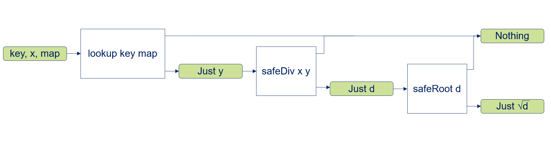
In each single step we have to check for Nothing, in that case we directly short circuit to an overall Nothing result value.
In the Just case we proceed to the next processing step.
This kind of handling is repetitive and buries the actual intention under a lot of boilerplate. As Haskell uses layout (i.e. indentation) instead of curly brackets to separate blocks the code will end up in what is called the dreaded staircase: it marches to the right of the screen.
So we are looking for a way to improve the code by abstracting away the chaining of functions that return
Maybe values and providing a way to short circuit the Nothing cases.
We need an operator andThen that takes the Maybe result of a first function
application as first argument, and a function as second argument that will be used in the Just x case and again
returns a Maybe result.
In case that the input is Nothing the operator will directly return Nothing without any further processing.
In case that the input is Just x the operator will apply the argument function fun to x and return its result:
andThen :: Maybe a -> (a -> Maybe b) -> Maybe b
andThen Nothing _fun = Nothing
andThen (Just x) fun = fun x
We can then rewrite findDivRoot as follows:
findDivRoot'''' x key map =
  lookup key map `andThen` \y ->
  safeDiv x y    `andThen` \d ->
  safeRoot d
(Side note: In Java the Optional type has a corresponding method: Optional.flatmap)
This kind of chaining of functions in the context of a specific data type is quite common. So, it doesn’t surprise us that
there exists an even more abstract andThen operator that works for arbitrary parameterized data types:
(>>=) :: Monad m => m a -> (a -> m b) -> m bWhen we compare this bind operator with the type signature of the andThen operator:
andThen :: Maybe a -> (a -> Maybe b) -> Maybe bWe can see that both operators bear the same structure.
The only difference is that instead of the concrete type Maybe the signature of (>>=)
uses a type variable m with a Monad type class constraint. We can read this type signature as:
For any type m of the type class Monad the operator (>>=) is defined as m a -> (a -> m b) -> m b
Based on (>>=) we can rewrite the findDivRoot function as follows:
findDivRoot' x key map =
  lookup key map >>= \y ->
  safeDiv x y    >>= \d ->
  safeRoot d
Monads are a central element of the Haskell type class ecosystem. In fact the monadic composition based on (>>=) is so
frequently used that there exists some specific syntactic sugar for it. It’s called the do-Notation.
Using do-Notation findDivRoot looks like this:
findDivRoot''' x key map = do
  y <- lookup key map
  d <- safeDiv x y
  safeRoot d
This looks quite like a sequence of statements (including variable assignments) in an imperative language. Due to this similarity Monads have been aptly called programmable semicolons. But as we have seen: below the syntactic sugar it’s a purely functional composition!
Purity
A function is called pure if it corresponds to a function in the mathematical sense: it associates each possible input value with an output value, and does nothing else. In particular,
- it has no side effects, that is to say, invoking it produces no observable effect other than the result it returns; it cannot also e.g. write to disk, or print to a screen.
- it does not depend on anything other than its parameters, so when invoked in a different context or at a different time with the same arguments, it will produce the same result.
Purity makes it easy to reason about code, as it is so close to mathematical calculus. The properties of a Haskell program can thus often be determined with equational reasoning. (As an example I have provided an example for equational reasoning in Haskell).
Purity also improves testability: It is much easier to set up tests without worrying about mocks or stubs to factor out access to backend layers.
All the functions that we have seen so far are all pure code that is free from side effects.
So how can we achieve side effects like writing to a database or serving HTTP requests in Haskell?
The Haskell language designers came up with a solution that distinguishes Haskell from most other languages: Side effects are always explicitly declared in the function type signature. In the next section we will learn how exactly this works.
Explicit side effects with the IO Monad
Monadic I/O is a clever trick for encapsulating sequential, imperative computation, so that it can “do no evil” to the part that really does have precise semantics and good compositional properties.
The most prominent Haskell Monad is the IO monad. It is used to compose operations that perform I/O.
We’ll study this with a simple example.
In an imperative language, reading a String from the console simply returns a String value (e.g. BufferedReader.readline() in Java:
public String readLine() throws IOException).
In Haskell the function getLine does not return a String value but an IO String:
getLine :: IO StringThis could be interpreted as: getLine returns a String in an IO context.
In Haskell, it is not possible to extract the String value from its IO context (In Java on the other hand you could always
catch away the IOException).
So how can we use the result of getLine in a function that takes a String value as input parameter?
We need the monadic bind operation (>>=) to do this in the same as we already saw in the Maybe monad:
-- convert a string to upper case
strToUpper :: String -> String
strToUpper = map toUpper

up :: IO ()
up =
  getLine >>= \str ->
  print (strToUpper str)

-- and then in GHCi:
λ> :t print
print :: Show a => a -> IO ()
λ> up
hello world
"HELLO WORLD"
or with do-Notation:
up' :: IO ()
up' = do
  str <- getLine
  print (strToUpper str)
Making side effects explicit in function type signatures is one of the most outstanding achievements of Haskell. This feature will lead to a very rigid distinction between code that is free of side effects (aka pure code) and code that has side effects (aka impure code).
Keeping domain logic pure - particularly when working only with total functions - will dramatically improve reliability and testability as tests can be run without setting up mocks or stubbed backends.
It’s not possible to introduce side effects without making them explicit in type signatures.
There is nothing like the invisible Java RuntimeExceptions.
So you can rely on the compiler to detect any violations of a rule like “No impure code in domain logic”.
I’ve written a simple Restaurant Booking REST Service API that explains how Haskell helps you to keep domain logic pure by organizing your code according to the ports and adapters pattern.
The section on type classes (and on Monads in particular) have been quite lengthy. Yet, they have hardly shown more than the tip of the iceberg. If you want to dive deeper into type classes, I recommend The Typeclassopedia.
Conclusion
We have covered quite a bit of terrain in the course of this article.
It may seem that Haskell has invented an intimidating mass of programming concepts. But in fact, Haskell inherits much from earlier functional programming languages.
Features like first class functions, comprehensive list APIs or declarative programming had already been introduced with Lisp and Scheme.
Several others, like pattern matching, non-strict evaluation, immutability, purity, static and strong typing, type inference, algebraic data types and polymorphic data types have been invented in languages like Hope, Miranda and ML.
Only a few features like type classes and explicit side effects / monadic I/O were first introduced in Haskell.
So if you already know some functional language concepts, Haskell shouldn’t seem too alien to you. For developers with a background in OO languages, the conceptual gap will be much larger.
I hope that this article helped to bridge that gap a bit and to better explain why functional programming - and Haskell in particular - matters.
Using functional programming languages - or applying some of their techniques - will help to create designs that are closer to the problem domain (as intented by domain driven design), more readable (due to their declarative character), allow equational reasoning, will provide more rigid separation of business logic and side effects, are more flexible for future changes or extensions, provide better testability (supporting BDD, TDD and property based testing), will need much less debugging, are better to maintain and, last but not least, will be more fun to write.